Handling of data gaps within files
When computing the spectra and amplitude levels, we read input files from the sds-directory one by one. The raw data may contain gaps however. If that is the case, we preserve the gaps by setting the affected windows to Nan so that they become Nans in the output as well.
In the following, the details of this processing are shown.
[1]:
import numpy as np

from scipy.signal import welch
from obspy.signal.filter import bandpass
[2]:
from obspy.clients.filesystem.sds import Client
from obspy.clients.fdsn import RoutingClient
from obspy.core import UTCDateTime as UTC
from obspy import read_inventory
[3]:
import matplotlib.pyplot as plt
plt.style.use('tableau-colorblind10')
[4]:
from data_quality_control import base, util
[5]:
from importlib import reload
[6]:
network = 'GR'
station = 'BFO'
location = ''
channel = 'BHZ'
overlap = 60 #3600

fmin, fmax = (4, 9.9)
nperseg = 2048
winlen_in_s = 3600
proclen = 24*3600

sds_root = '../sample_sds/' #'/sds/'
inventory_routing_type = 'eida-routing'

sdsclient = Client(sds_root)
invclient = RoutingClient(inventory_routing_type)
[7]:
starttime = UTC("2020-360")
#overlap = 600
[8]:
#reload(processing)
processor = base.NSCProcessor(
        network,
        station,
        location,
        channel,
        dataclient=sdsclient,
        invclient=invclient,)
using default for overlap
using default for amplitude_frequencies
using default for nperseg
using default for winlen_seconds
using default for proclen_seconds
using default for sampling_rate
Obtain waveforms from SDS.
[9]:
starttime = starttime - overlap
endtime = starttime + proclen + 2*overlap
st = sdsclient.get_waveforms(starttime=starttime,
                             endtime=endtime,
                    **processor.nsc_as_dict())

print(st)
1 Trace(s) in Stream:
GR.BFO..BHZ | 2020-12-25T00:00:02.369538Z - 2020-12-26T00:01:00.019538Z | 20.0 Hz, 1729154 samples
The data originally does not contain any gaps. Otherwise there would be multiple traces in the stream. We simulate missing data by cutting out some hours of this trace:
[10]:
st = st.cutout(starttime+6*3600+900, starttime+9*3600+1800)
print(st)
2 Trace(s) in Stream:
GR.BFO..BHZ | 2020-12-25T00:00:02.369538Z - 2020-12-25T06:14:00.019538Z | 20.0 Hz, 448754 samples
GR.BFO..BHZ | 2020-12-25T09:29:00.019538Z - 2020-12-26T00:01:00.019538Z | 20.0 Hz, 1046401 samples
Obtain corresponding inventory from RoutingClient.
[11]:
inv = invclient.get_stations(starttime=starttime,
                        endtime=endtime, level='response',
                        **processor.nsc_as_dict())
/home/docs/checkouts/readthedocs.org/user_builds/lonesam/conda/latest/lib/python3.9/site-packages/obspy/io/stationxml/core.py:96: UserWarning: The StationXML file has version 1.2, ObsPy can read versions (1.0, 1.1). Proceed with caution.
  warnings.warn("The StationXML file has version %s, ObsPy can "
Process data, i.e. remove sensitivity to obtain ground velocity.
[12]:
tr = util.process_stream(st, inv,
            starttime, endtime, sampling_rate=20)
print(tr)
GR.BFO..BHZ | 2020-12-24T23:59:00.019538Z - 2020-12-26T00:00:59.969538Z | 20.0 Hz, 1730400 samples
[13]:
tr.plot(show=False)
[13]:

Obviously the trace now contains a large data gap.
[14]:
np.where(np.isnan(tr.data))
[14]:
(array([ 0, 1, 2, ..., 683997, 683998, 683999]),)
Now, let’s go through the routine that extracts the spectra and amplitudes step by step.
[15]:
# Get some numbers
sr = tr.stats.sampling_rate
nf = int(proclen/winlen_in_s)
#proclen_samples = proclen * sr
winlen_samples = int(winlen_in_s * sr)
For the spectra, we can simply reshape the data within the time which we want to analyse. It’s the time window minus the overlaps at the end, so starttime+overlap and endtime-overlap.
[16]:
# Data for spectra computation
data = util.get_adjacent_frames(tr,
        starttime+overlap, nf, winlen_samples)
Let’s take a look at the data matrix:
Rows show 1 h of data.
Between 6:15 and 9:30 is a data gap in which data is Nan.
[17]:
plt.imshow(data, aspect='auto')
plt.ylabel('hours')
plt.xlabel('npts');

[18]:
scale = 1e6
for i, row in enumerate(data):
    plt.plot(row*scale + i)
plt.ylabel('hours')
plt.xlabel('npts');

Spectra are only computed for rows without Nans. So the resulting array with the spectral data looks like this:
[19]:
freq, P = welch(data, fs=sr, nperseg=nperseg, axis=1)
[20]:
plt.imshow(np.log(P), aspect='auto')
plt.ylabel('hours')
plt.xlabel('npts');

[21]:
i, j = np.where(np.isnan(P))
print(np.unique(i))
[0 6 7 8 9]
For the amplitudes, we want to get the \(p\)-th percentile of each time frame (e.g. 1 h) in the data. We use np.percentile. In principle, we need the data again as a 2d-array with rows corresponding to each time frame, as it was the case for the spectral computation.
However, for the extraction of amplitude informations, the situation is a little more complicated because we want to filter the data.
To avoid edge effects from filtering affecting the amplitude extraction, we need want the data to be a little bit longer than needed. This is why we add some overlap to the ends of the requested time window.
For contiguous data, we can simply filter the entire trace at once, cut off the overlap and reshape the data vector into a 2d array as for the spectral computation.
Unfortunately, the filter function stops at the first occurrence of Nans. So in the example, we would only get amplitudes for the first 4 hours, even though later, several complete hours are left, that could be analysed.
Thus, if Nans are present, we filter the data frame-wise. However, to accomodate the edge effects, we need some overlap between the frames as well. The overlap gets tapered by multiplying each frame with a Tukey window. Then, we filter each row and for the amplitude analysis, we then just use the inner, non-tapered part.
The decision, which workflow to use, is made by processing.get_amplitude.
Let’s take a look at these steps:
First, we take a look at what happens, if we use simple, adjacent frames and filter them.
[22]:
# Reshape into frames
data = util.get_adjacent_frames(tr,
        starttime+overlap, nf, winlen_samples)

# Filter row-wise
filtered1 = bandpass(data.copy(), fmin, fmax, sr)
The next plot demonstrates, how the filter function bandpass reacts if Nans are in a row:
The row at 5:00 is processed until the first occurrence of Nans after around 250000 samples.
The row at 9:00 is not processed at all, although we know from the figures above of the unfiltered data that the data returns later in that hour.
[23]:
scale = 5e6
for i, row in enumerate(filtered1):
    plt.plot(row*scale + i)
plt.ylabel('hours')
plt.xlabel('npts');
#plt.xlim(-10, 100)

If we zoom in at the beginning of the rows, we see the edge effects of the filter. That’s the high amplitude wiggle at the beginning.
[24]:
scale = 1e8
for i, row in enumerate(filtered1):
    plt.plot(row*scale + i, lw=1)
plt.ylabel('hours')
plt.xlabel('npts');
plt.xlim(-100, 10000)
plt.ylim(0, 25);

Compare it with the unfiltered beginnings. There is no such overshoot in the data.
[25]:
scale = 1e6
for i, row in enumerate(data):
    plt.plot(row*scale + i)
plt.ylabel('hours')
plt.xlabel('npts');
plt.xlim(-100, 10000)
plt.ylim(0, 25);

So for the amplitude analysis, we want to exclude this early part. But if we do this now, we could only analyse slightly less than our desired frame length of 1 hour.
This is why we here need overlapping frames.
[26]:
taper_samples = int(overlap*sr)
data2, taper = util.get_overlapping_tapered_frames(
        tr.copy(), starttime+overlap, nf, winlen_samples,
        taper_samples)
Note that the data matrix is now slightly bigger than for the simple, adjacent framing, namely twice the taper length.
[27]:
print('simple frames', data.shape)
print('overlapping frames', data2.shape)
simple frames (24, 72000)
overlapping frames (24, 74400)
If we now apply the filter row-wise, the edge effects are suppressed by the taper. The frame that we actually want to use, starts after the fade-in. The same occurs of course at the other end.
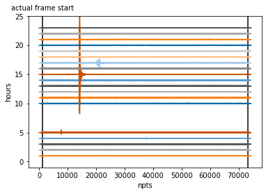
[28]:
# Filter row-wise
filtered2 = bandpass(data2.copy(), fmin, fmax, sr)
[29]:
scale = 1e8
for i, row in enumerate(filtered2):
    plt.plot(row*scale + i)
plt.vlines(taper, -1, 25, 'k')
plt.text(taper, 26, 'actual frame start',
         ha='center')
plt.ylabel('hours')
plt.xlabel('npts');
plt.xlim(-100, 10000)
plt.ylim(-1, 25);

util.get_overlapping_tapered_frames also sets all rows containing any Nans to Nan entirely.
[30]:
scale = 1e7
for i, row in enumerate(filtered2):
    plt.plot(row*scale + i)
plt.vlines([taper, filtered2.shape[1]-taper],
           -1, 25, 'k')
plt.text(taper, 26, 'actual frame start',
         ha='center')
plt.ylabel('hours')
plt.xlabel('npts');
#plt.xlim(-10, 1000)
plt.ylim(-1, 25);
Thus, we can apply np.percentile to the targeted section filtered2[:,taper:-taper] to get es
[31]:
perc = 75
[32]:
prctl = np.percentile(filtered2[:,taper:-taper],
                      perc, axis=1)
and compare it with the result of util.get_amplitude which summarizes the previous steps.
[33]:
prctl_direct = util.get_amplitude(
        tr, starttime+overlap,
            fmin, fmax, overlap, winlen_samples, nf)
24-02-09 13:26:45 - data_quality_control.util - INFO - Found nans in GR.BFO..BHZ | 2020-12-24T23:59:00.019538Z - 2020-12-26T00:00:59.969538Z | 20.0 Hz, 1730400 samples
/home/docs/checkouts/readthedocs.org/user_builds/lonesam/conda/latest/lib/python3.9/site-packages/numpy/lib/nanfunctions.py:1395: RuntimeWarning: All-NaN slice encountered
  result = np.apply_along_axis(_nanquantile_1d, axis, a, q,
The RuntimeWarning regarding All-NaN slices is issued by numpy.nanquantile() and can be ignored. It occurs when the subarray (a row in our case) to which the operator is applied contains only Nans. This is however expected and intended as there is simply no data for several hours.
[34]:
plt.plot(prctl, 'o:', ms=10,
         label='prctl (step by step)')
plt.plot(prctl_direct, 's:', ms=5,
         label='prctl_direct (processing.get_amplitudes()')
[34]:
[<matplotlib.lines.Line2D at 0x7f03cfbc0490>]

Difference:
[35]:
prctl-prctl_direct
[35]:
array([ nan,   0.,   0.,   0.,   0.,   0.,  nan,  nan,  nan,  nan,   0.,
         0.,   0.,   0.,   0.,   0.,   0.,   0.,   0.,   0.,   0.,   0.,
         0.,   0.])
Note on tr.slice / tr.trim
However, using time objects at both ends can result in a bad number of samples. This is because the demanded times may not fall exactly at the samples in the trace. In this case obspy has to choose where to set the cut. As a result, the number of samples in a trace can vary by 1 or 2 for the same time length.
Since we want to apply np.reshape we need the total number of samples in the vector (our data) to be exactly \(n_{tot} = n_{frames} \times n_{win}\) with \(n_{win}\) being the number of samples per frame, so length of frame in seconds \(l\) times sampling rate \(f\): \(n_{win} = l \times f\)
Therefore, we just use the starttime and then select \(n_{tot}\) samples.
[ ]: